Introduction

It is common to say that “Everything is a System” or even “a System-of-Systems”, but the consequences of that are becoming increasingly alarming to the energy industry. In cases from the earthquake-triggered Fukushima disaster to (possible) foreign hacking of the electrical grid, the vulnerabilities of the energy supply to the physical, economic and political domains are obvious.

An effective approach to prediction and preparation requires that our models be as integrated as the systems they represent. Here, the object-oriented nature of SysML provides a major benefit. In this blog post, we look at the integration of models of widely different scale and subject.

The case study in Part 1 was primarily about design and touched only briefly on analysis. However, analysis is a critical part of MBE and should be incorporated into the system model as early as possible to:

• evaluate possible system variants
• explore system risk
• verify requirements on an ongoing basis

Generally, complex systems require many different kinds of analytical models, and analytical models applied to separate subsystems must be confederated to analyze the total system.

Case Study 2: Energy System Analysis

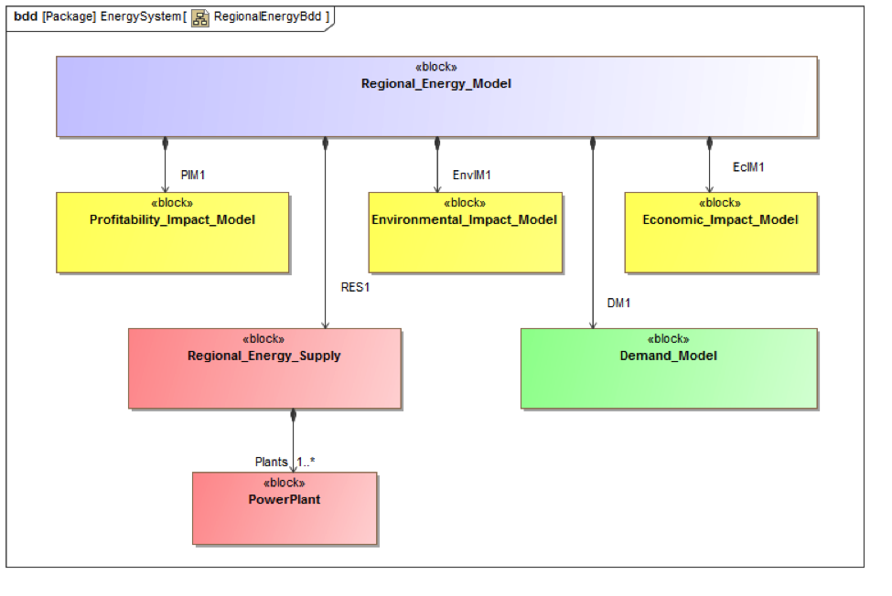
In this case study, we look at how some of these issues play out in modeling a regional energy system. In Figure 1, we consolidated several analytical models into a single structure in SysML.

• • The power plant models calculate cost of power generation as a function of capital, fixed operating and variable operating costs, and an environmental cost associated with emissions (solid, liquid, gaseous and capacity build). These blocks could contain models like the one developed in the first case study.
    

    Figure 1 Regional Energy Model block definition diagram, Phase

• • A Regional Energy Supply model consolidates the supply models and calculates weighted average costs

• • An aggregate Demand model based on standard price elasticity

• Profit, Economic Impact and Environmental Impact models that evaluate the effect of supply and demand values on the utility and the region.

In our study, these models used SysML parametric diagrams to connect parameters and constraints. Some of these models use MATLAB and Mathematica functions. Common parameters such as supply (MW), demand (MW), cost ($/kW-hr) and price ($/kW-hr) are exchanged through the top-level Regional_Energy_Model block.

In other projects, Intercax has developed other SysML analysis models evaluating, for example, Smart Grid and Smart Home systems. In the Smart Grid model, the utility distribution system has been built to provide price information to consumers, some of whom have the ability to shift demand to low price periods during the day. In the Phase 2 diagram in Figure 2, we add new blocks to the models, including the Distribution and SmartGrid Demand models, from that project.

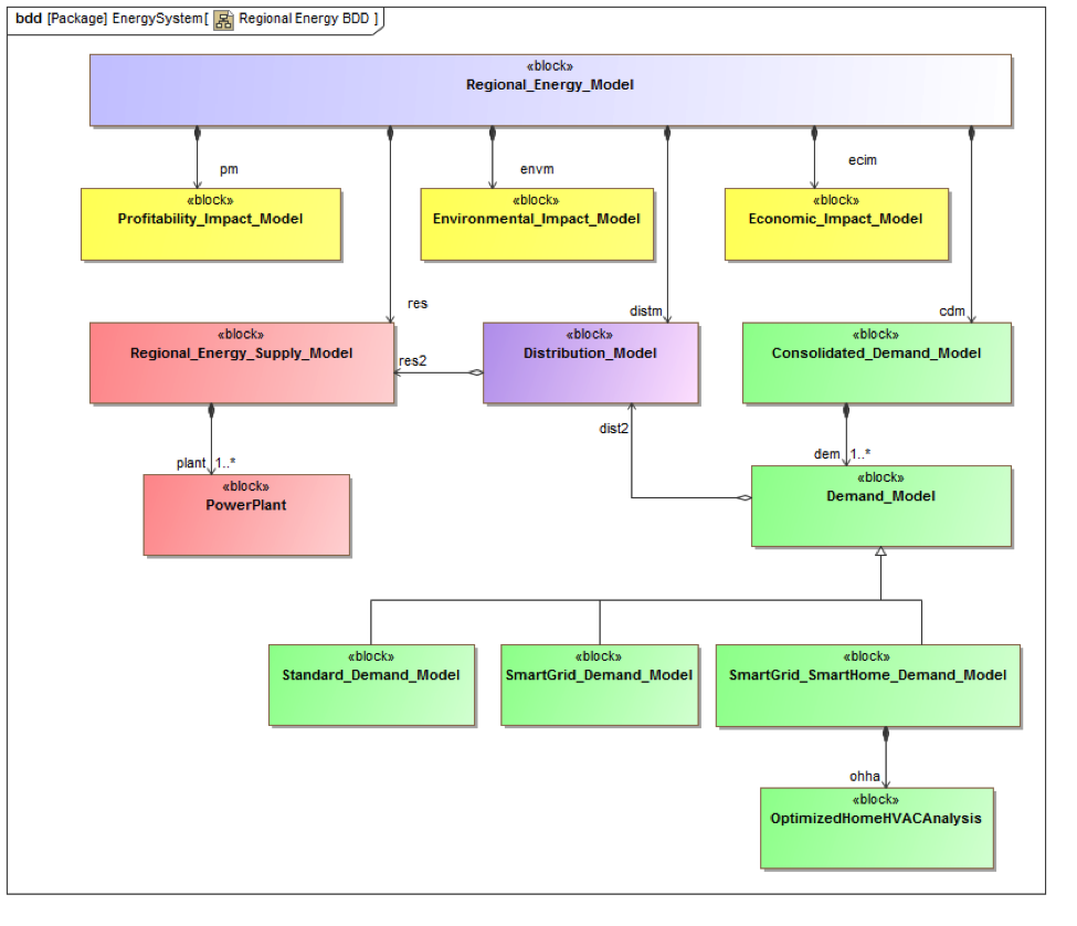
Figure 2 Regional Energy Model block definition diagram, Phase 2

The SmartHome project explored the use of the “Internet of Things” to reduce demand in a networked residential user, by, for example, reducing HVAC activity when parts of the home were unoccupied. The SysML reference model for the SmartHome, had its own analysis, OptimizedHomeHVACAnalysis. This top-level analysis block is used directly by the SmartGrid_SmartHome_Demand model at the bottom right in Figure 2.

When the model in Figure 2 is instantiated, we can readily choose a combination of different sources and consumers. In one example, we chose a combination of three generation facilities (coal-fired, nuclear and solar), each with time-dependent supply and cost values (considered in one-hour intervals over a twenty-four hour cycle). We chose three different combinations of demand models, with a constant base demand schedule underlying different levels of price elasticity, demand shift elasticity and demand reduction, depending on their adoption of SmartGrid and SmartHome technologies.

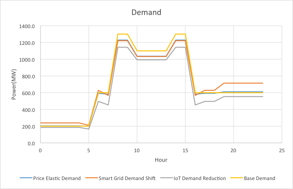
Figure 3 Demand curve shifts reflecting price elasticity, demand shift and demand reduction

Figure 3 shows the results of these calculations by hour of the day for a combination of industrial and residential demand. Price elasticity reduces demand, especially at the most expensive midday rates when consumption is highest and demand shift elasticity has the highest impact for residential customers in the late night and early morning hours, but relatively little for industrial demand which is confined to midday hours in our model.

The objective of this exercise is not to claim that the specific models used here reflect accurate usage predictions, but to show how readily an MBE approach with an object-oriented language like SysML allows federation of diverse multidisciplinary models.

The Future of MBE for Energy Applications

Executable versions of the Regional Energy Demand SysML models can be downloaded for inspection (all are copyrighted by Intercax LLC and can be with permission). To execute them requires one of the parametric solver plug-ins from Intercax, as well as one or more solver engines such as Mathematica or MATLAB. See the product description pages on our website for more information.

Parts 1 and 2 of this series have focused on the SysML models. In Part 3, we will describe the MBE graphs created when the SysML model is connected to all the other engineering models used in these efforts. In particular, we will focus on how to visualize and query the graphs, with the ultimate objective of identifying connections that throw light on the reliability or resilience of the system.

SysML Models

• Regional_Energy_Model_Example.mdzip
• RegionalEnergyModel_RHP.zip

Related posts:

• MBE for the Energy Industry | Part 1
• MBE for the Energy Industry | Part 2 (this post)
• MBE for the Energy Industry | Part 3

Tweet